a-algorithm

A* Search Algorithm

What is an A* search algorithm?

• In A Level Computer Science, the A* algorithm builds on Dijkstra’s by using a heuristic

• A heuristic is a rule of thumb, best guess or estimate that helps the algorithm accurately approximate the shortest path to each node

• Dijkstra’s shortest path algorithm is an example of a path-finding algorithm. Other path finding algorithms exist that are more efficient. One example is the A* search

• Dijkstra’s uses a single cost function i.e. the weight of the current path plus the total weight of the path so far. This is the real distance from the initial node to every other node

• To revise Graphs you can follow this link

• The cost function is unreliable, for example, going from node A to B may be a large distance such as 117, whereas going from A to C may be a distance of 5. Dijkstra’s will follow node C even if it doesn’t lead to the goal node as A to C is simply the shortest path

• In order to prevent going in the wrong direction, another function is necessary: a heuristic function

• A* search uses g(x) as the real distance cost function and h(x) as the heuristic function

• Every node will have a heuristic value. The purpose of the heuristic function is that it will approximate the Euclidean distance i.e. the straight line distance from the current node to the goal node. By following nodes based on shorter heuristic distances, the algorithm can be sure it is getting closer to the goal node

• As the heuristic is an estimate, it is not necessarily optimum. The A* search operates under the assumption that the heuristic function should never overestimate the real cost from the initial node to the goal node. The real cost should always be greater or equal to the heuristic function

• The total cost f(x) of each node rather than just g(x) (the distance from node X to Y plus the previous route total distance) is g(x) + h(x) (the estimate of how far the goal node is away from the current node)

  • The calculation for each node is therefore f(x) = g(x) + h(x)

  • If h(x) increases compared to the previous node, it means the algorithm is traveling further away from the goal node

• A* search focuses on reaching the goal node unlike Dijkstra’s which calculates the distance from the initial node to every other node

• Below is an illustration of the A* search

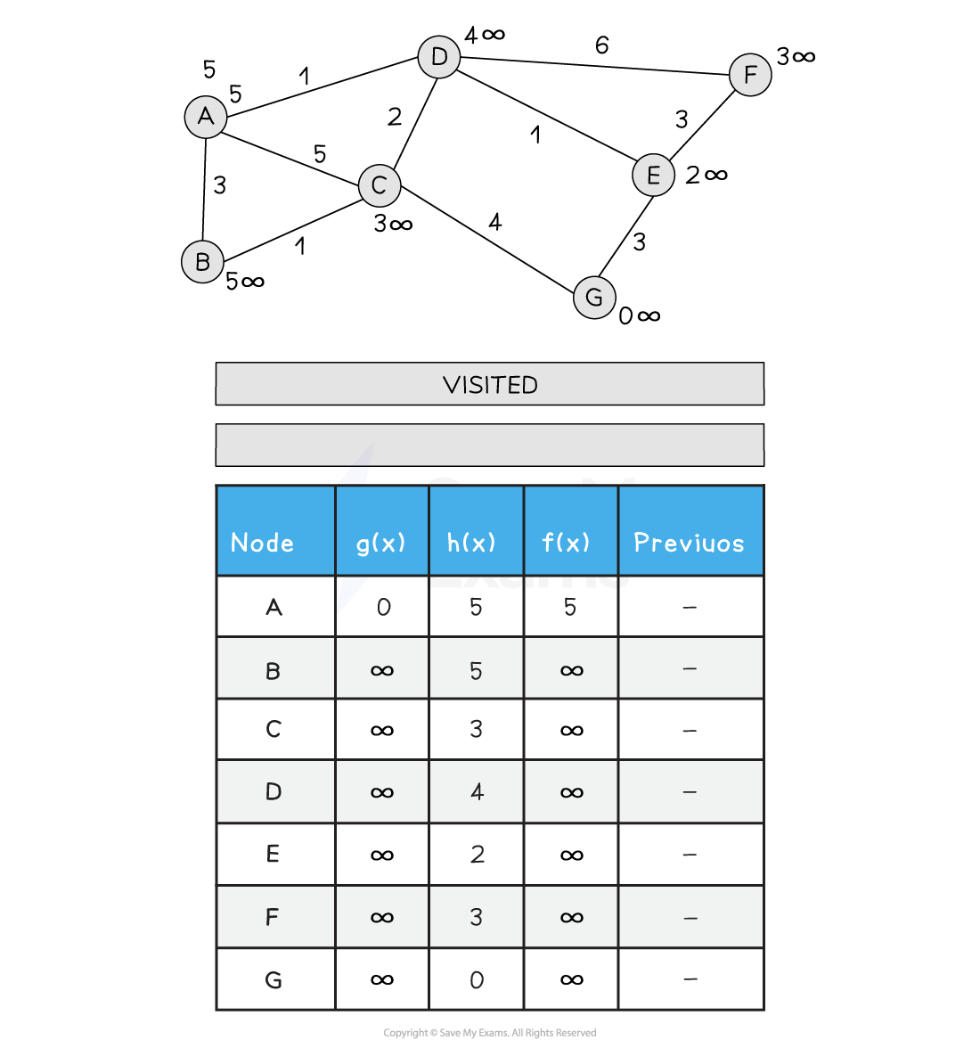
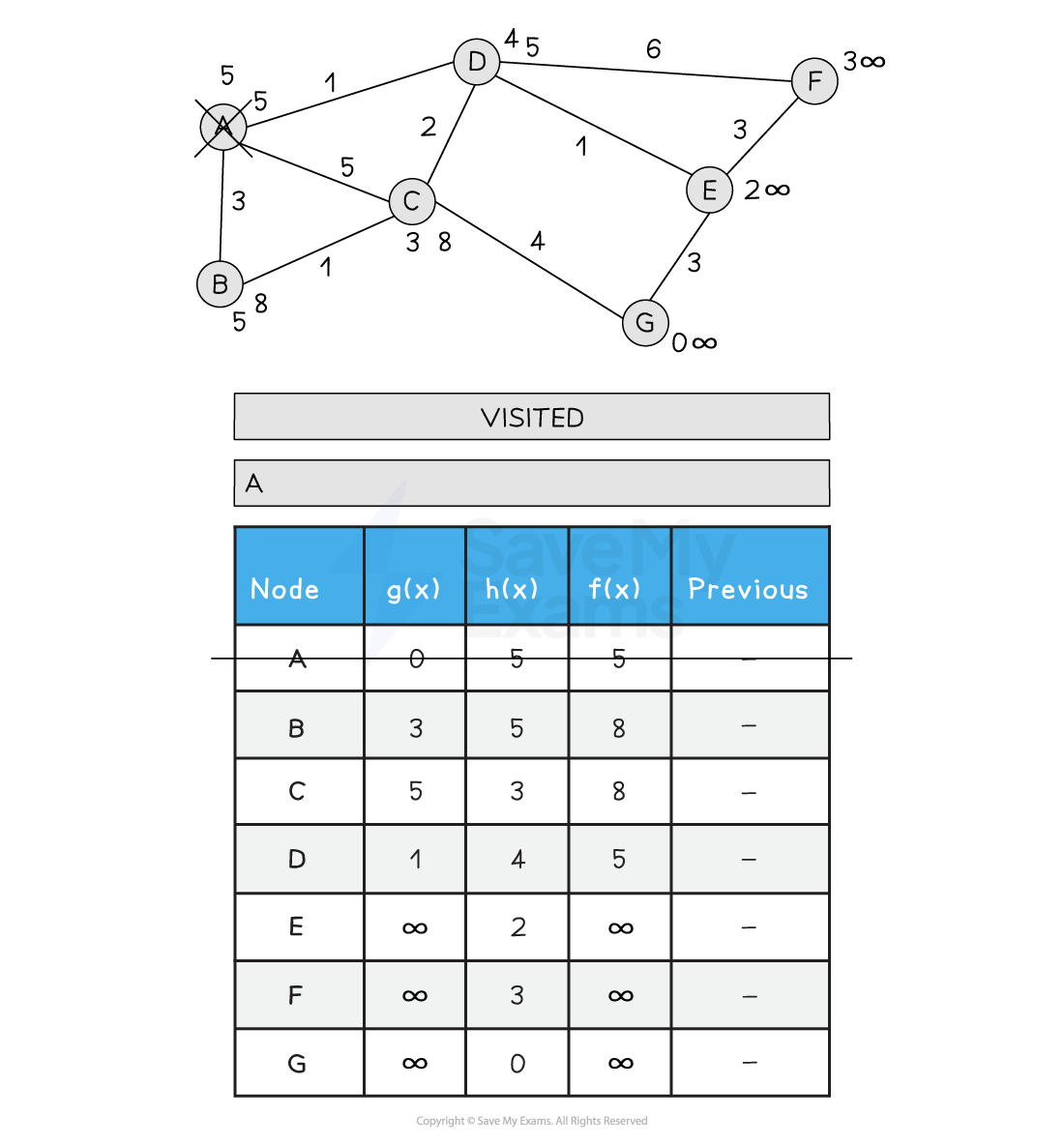
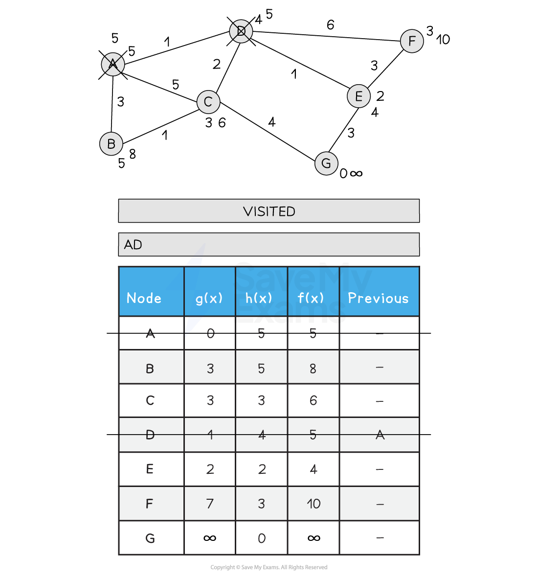
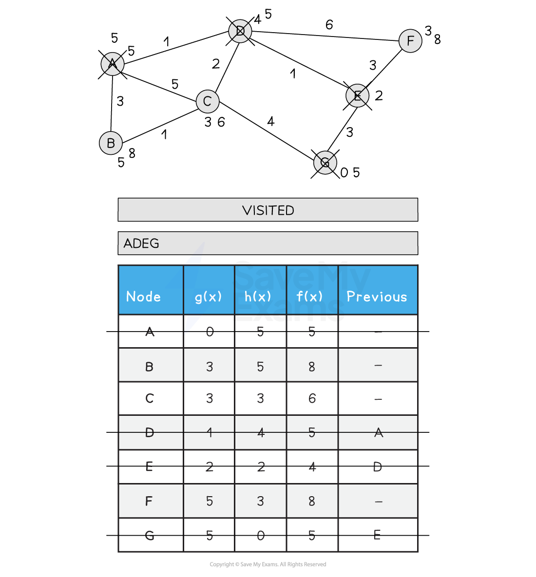
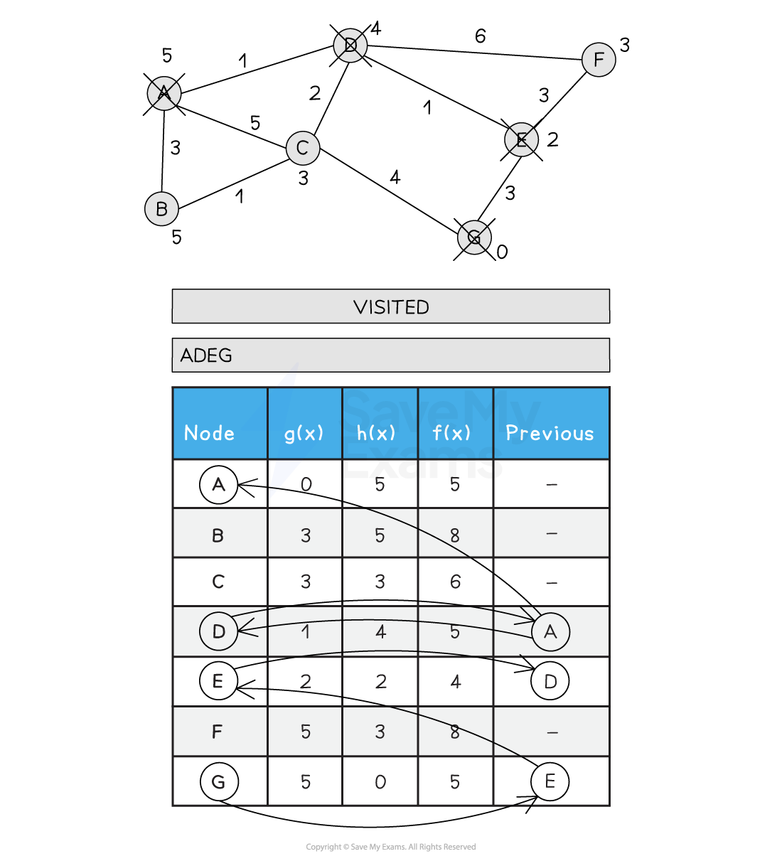
Figure 2: Performing the A* Search

• The algorithm for A* search is shown below, both in structured english and a pseudocode format

A* Search (Structured English)

assign g(x) to 0 and f(x) to h(x) for the initial node and g(x) and f(x) to infinity for every other node
add all nodes to a priority queue, sorted by f(x)
while the queue is not empty remove node x from the front of the queue and add to a visited list If node x is the goal node,
end the while loop else for each unvisited neighbour y of the current node x g(x) = g(x)AtX + distanceFromXtoY if g(x) < g(x)AtY then g(x)AtY = g(x) f(x)AtY = g(x)AtY + h(x)AtY reorder the priority queue by changing Y’s position based on the new f(x) endif next X
endwhile

A* Search (Pseudocode)

function AStarSearch(graph, start, goal) //set all distances to infinity and first distance to 0
for node in graph g[node] = infinity f[node ] infinity next node g[start] = 0 f[start] = h[start] //A* ends when the goal node has been reached while goal in graph //find the shortest distance f(x) from all the nodes in order to select the next node to visit and expand min = null for node in graph If min == null then min = node elseif f[node] < f[min] then min = node endif next node //for each neighbour, update the cost if the current cost and distance are less than the previously stored distance for neighbour in graph if cost + distance[min] < distance[neighbour] then distance[neighbour] = cost + distance[min] F[neighbour] = cost + g[min] + h[neighbour] previousNode[neighbour] = min endif next neighbour graph.remove(min) endwhile //backtrack through the previous nodes and build up the final path until the start is reached node = goal
while node != start path.append(node) node = previousNode[node]
endwhile return path endfunction

• A* search behaves almost exactly as Dijsktra’s except that when the goal node is reached, the algorithm stops and the old cost function is replaced with a new heuristic based function

Tracing the A* Search Algorithm

• Tracing the A* search algorithm can be done in a manner similar to the Figure 2 above

• Remember to initialise the starting node g(x) to 0 and f(x) to h(x)

• Update each nodes neighbours by adding the previous path and the distance from the current node to the neighbour to the heuristic value for the neighbour node

• Keep track of each nodes previous node that offered the shortest route